Contents
Calculator Tutorial
1.1 Adding items to an equation
1.2 Moving and deleting items in an equation
1.3 Interpreting The Solution
1.4 Exporting The Equation
1.5 Using The Graph
1.6 Changing The Settings
About Matrices
2.1 Introduction to Matrices
2.2 Addition and Subtraction
2.3 Transpose
2.4 Multiplication
2.5 Matrix-Scalar Product
2.6 Dot-Product
2.7 Matrix-Matrix Product
2.8 Determinant
2.9 Inverse
1.1 Adding items to an equation
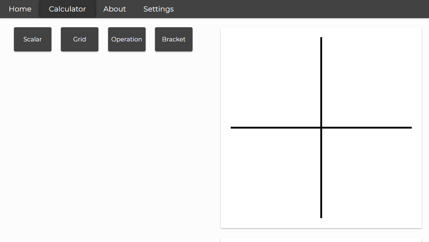
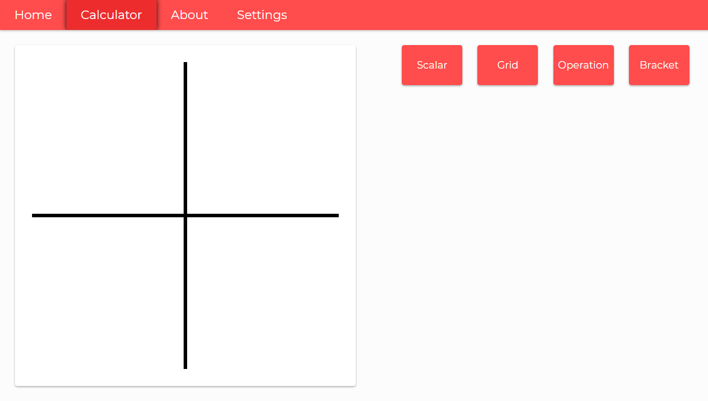
To create an equation, you can use the row of bottoms near the top of the calculator page.Each of these buttons adds a different type of mathematical item to the equation:
- Scalar - A single number (can be integer or decimal).

- Grid - A grid of scalars (if 1 column, it represents a vector, otherwise it represents a matrix).
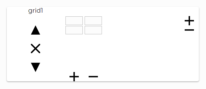
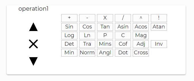
- Operation - A mathematical operation that takes a set of operands and produces an output e.g. add, multiply, sine, factorial etc.
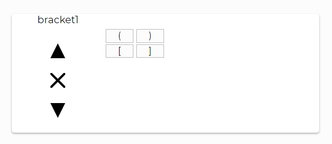
- Bracket - A symbol that encloses a set of items, chaning the way they are evaluated.
An equation should be formed, where from top to bottom of the screen represents left to right in conventional mathematical notation e.g:
Scalar (2)
Operation (+)
Scalar (5)
Is interpreted as:
2 + 5
1.2 Moving And Deleting Items In An Equation
Move item:
Once you have added an item to an equation and now wish to change its position, you can do so using the up/down arrows on the left side of each item.
Delete item:
Alternatively, if you wish to remove an item entirely, you can use the cross button between the two movement arrows.

Delete all items:
To remove all the items from equation, press the 'clear' button at the bottom of the equation.
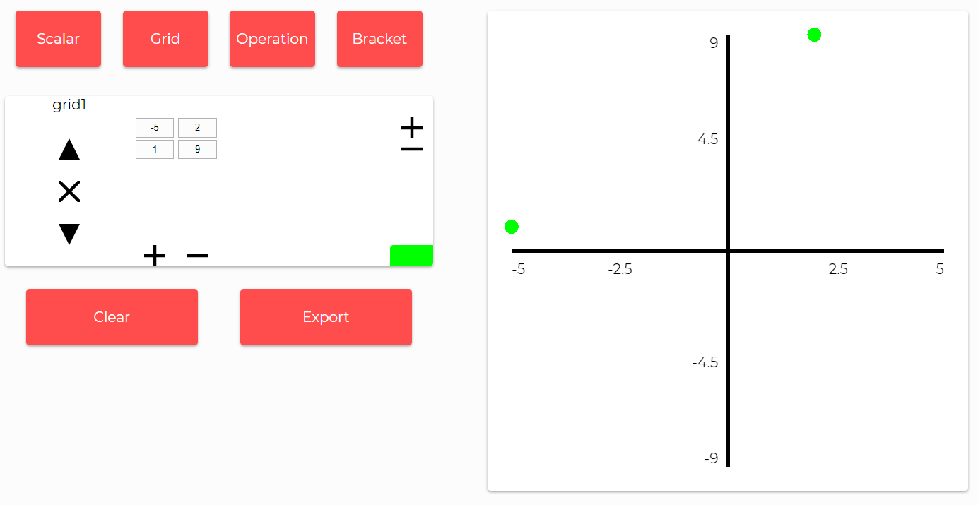
1.3 Interpreting The Solution
As soon as you begin adding items to the equation, the calculator will attempt to evaluate the equation you have input.
The solution will be displayed in a small box underneath the graph.
If the equation (or solution to it) does not involve any 2 x n matrices, the graph will be blank.
When evaluating an equation, there are 3 possible outcomes:
- Empty Equation - There are no items in the equation for the calculator to evaluate.
- Parse failed - The calculator could not understand the input you gave it. Check all text boxes are filled, and all items (e.g. operations and brackets) have a type selected.

- Solve failed - The equation was understood, but no solution could be found. Check for errors with the maths e.g. division by 0, or unclosed brackets.

- [Solution given] - The calculator was able to evaluate the input equation to give a solution. It should be displayed in correct mathematical notation (using LaTeX).

If the solution is a 2 x n matrix/vector, it will be displayed on the graph with a unique color (black by default).
1.4 Exporting The Equation
To save an equation and its solution + graph to a file, for viewing at a later date, we can use the export button below the main equation.

It will be generate a .html file that can be viewed in all web browsers, with a LaTeX representation of the equation.
Below it is the graph and all its points displayed as an image.
The exported file is not interactive, it can only be used for viewing, and not further calculation.
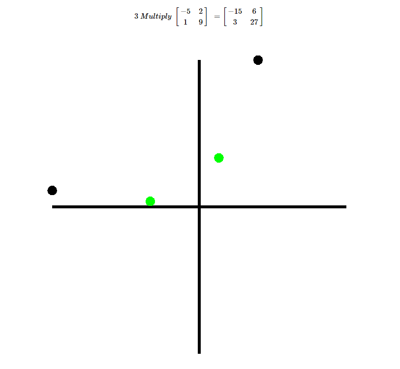
1.5 Using The Graph
The graph is used to display all matrices/vectors that are 2 dimensional. It will always scale to fit the largest matrix/vector it is displaying.
Any time a 2 dimensional matrix/vector appears, either in the equation or solution, it will be displayed onto the graph.

Each matrix/vector is assigned a unique color, which is indicated in the bottom right corner of the item box.
This is the color used when its points are displayed on the graph.
You can also hide/show a matrix by clicking once on the colour indicator. If it becomes faded, the points are hidden, however if it becomes bold colored points are visible.

1.6 Changing The Settings
The calculator can be customised to fit the users prefernces from within the settings page.
Here is an overview of the settings which can be edited:
- Color - The color used for many elements within the page e.g. the navbar, buttons, links.
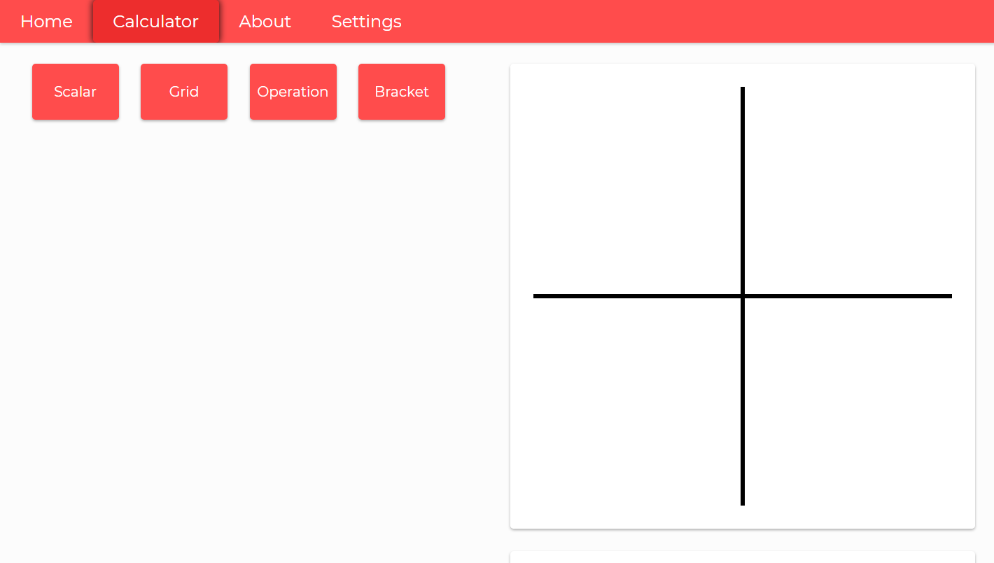
You have the following choice of colours to choose from:

- Shade - Use either a light or dark theme for elements on the page.

- Style - Choose between having shadows and rounded corners (material) or flat rectangles (flat).

- Calculator Layout - Decide the arrangement of the panels in the calculator page. You can either have the equation or the graph displayed on the left. (At the top if using a mobile device).
- Angle Unit - Choose between radians or degrees (used for trigonometric functions and angle between vectors).
2.1 Introduction To Matrices
A matrix is just a grid of numbers, like the following example of a 3x3 matrix:
$ \begin{bmatrix} 4 & 1 & 7 \\ 9 & 6 & 2 \\ 2 & 8 & 1 \\ \end{bmatrix} $
The "order" of a matrix is defined as the number of rows by the number of columns.
Often denoted m x n, the following is an example of a matrix of 2x4 order:
$ \begin{bmatrix} 4 & 6 & 0 & 9 \\ 6 & 3 & 2 & 8 \\ \end{bmatrix} $
Matrices with only one row or column are known as vectors.
This is an example of a column vector because it only has one column:
$ \begin{bmatrix} 3 \\ 8 \\ 1 \\ \end{bmatrix} $
And this is an example of a row vector, because it only has one row:
$ \begin{bmatrix} 6 & 2 & 5\\ \end{bmatrix} $
2.2 Addition and Subtraction
Matrices are treated differently to normal mathematical expressions, they are added, subtracted and multiplied in their own specific way.
Note that you cannot divide one matrix by another.
To add two matrices, you just add together the items in the same spaces, for example:
$ \begin{bmatrix} 1 & 3 \\ 6 & 4 \\ \end{bmatrix} + \begin{bmatrix} 5 & 9 \\ 1 & 7 \\ \end{bmatrix} = \begin{bmatrix} 6 & 12 \\ 7 & 11 \\ \end{bmatrix} $
Similarly, you can do the same process for subtraction, for example:
$ \begin{bmatrix} 8 & 0 \\ 6 & 1 \\ \end{bmatrix} - \begin{bmatrix} 2 & 1 \\ 3 & 7 \\ \end{bmatrix} = \begin{bmatrix} 6 & -1 \\ 3 & -6 \\ \end{bmatrix} $
2.3 Transpose
"Taking the transpose" means swapping all the rows for columns and columns for rows and is denoted by a capital T in superscript.
Here are some examples of taking the transpose:
$ \begin{bmatrix} 2 & 7\\ 1 & 5\\ \end{bmatrix} ^T = \begin{bmatrix} 2 & 1\\ 7 & 5\\ \end{bmatrix} $
For column vectors, this looks like the following:
$ \begin{bmatrix} 7\\ 3\\ 1\\ \end{bmatrix} ^T = \begin{bmatrix} 7 & 3 & 1\\ \end{bmatrix} $
And for row vectors it looks like so:
$ \begin{bmatrix} 2 & 8 & 5\\ \end{bmatrix} ^T = \begin{bmatrix} 2\\ 8\\ 5\\ \end{bmatrix} $
Note that transposing a matrix or vector twice, will give you back the original matrix/vector.
2.4 Multiplication
When it comes to multiplication, matrices are much more complicated than regular scalars.
There are multiple types of matrix multiplication including: matrix-scalar product, matrix-matrix product, dot-product, cross-product.
2.5 Matrix-Scalar Product
Multiplying a matrix by a scalar is very simple, for example:
$ 3 \cdot \begin{bmatrix} 3 & 9 \\ 5 & 1 \\ \end{bmatrix} = \begin{bmatrix} 9 & 27 \\ 15 & 3 \\ \end{bmatrix} $
2.6 Dot-Product
If you are multiplying with two column vectors, there is a method called "taking the dot product" in which you multiply together elements in corresponding rows and add this to the total.
After calculating dot product, you will get a single scalar value as an output:
$ \begin{bmatrix} 3\\ 2\\ 8\\ \end{bmatrix} \cdot \begin{bmatrix} 7\\ 4\\ 3\\ \end{bmatrix} = 21+8+24 = 53 $
If you need to calculate the dot product of a column vector and row vector, you must first transpose the row vector.
You can then calculate the dot product as usual:
$ \begin{bmatrix} 7\\ 1\\ 8\\ \end{bmatrix} \cdot \begin{bmatrix} 5 & 3 & 2\\ \end{bmatrix} ^T \\= \begin{bmatrix} 7\\ 1\\ 8\\ \end{bmatrix} \cdot \begin{bmatrix} 5\\ 3\\ 2\\ \end{bmatrix} \\= 35+3+16 \\= 52 $
2.7 Matrix-Matrix Product
Alternatively, when multiplying together two matrices, we use "matrix multiplication".
The following is the standard result for multiplying two 2x2 matrices:
$ \begin{bmatrix} a & b \\ c & d \\ \end{bmatrix} \cdot \begin{bmatrix} e & f \\ g & h \\ \end{bmatrix} \\= \begin{bmatrix} a \cdot e + b \cdot g & a \cdot f + b \cdot h \\ c \cdot e + d \cdot g & c \cdot f + d \cdot h \\ \end{bmatrix} $
Although it may be hard to see how this is derived, the process is really very simple:
1. Starting with the first row of the left matrix, take the dot product with the first column of the right matrix. Place this value in row 1 column 1 of the output matrix.
2. Next, take the dot product, but using the second column of the right matrix instead.
3. Continue this process for all columns in the right matrix.
4. Once you have done this, move on to the second row of the left matrix and repeat all the above steps.
5. Continue through all rows of the left matrix until you reach the end.
2.8 Determinant
Another property of a matrix is the determinant, which is also single scalar quantity.
The determinant of a matrix is generally denoted by two straight lines either side of it.
Here is an example of finding the determinant of a 3 x 3 matrix using the first column:
$ \begin{vmatrix} 9 & 5 & 1\\ 4 & 7 & 8\\ 2 & 3 & 4\\ \end{vmatrix} \\= 9(7 \cdot 4 - 8 \cdot 3) \\ \ \ - 4(5 \cdot 4 - 1 \cdot 3) \\ \ \ + 2(5 \cdot 8 - 1 \cdot 7) \\= 34 $
Note that the determinant only exists for a square matrix e.g. 3x3.
For any matrix, the process to find the determinant is as follows:
1. Starting from the first element of any row or column, remove from the matrix the row and column that element is on. For this example we will use the first row.
2. Using this entire process again, calculate the determinant of the smaller matrix left over (known as the minor matrix) and multiply this value by the original element you chose in step 1. Add the result to the total.
3. Move along to the next element in the row, and repeat the process. Instead of adding to the total however, you must subtract from it. You change whether you add or subtract every time you move along an element.
4. Once you have reached the end of the row. The total you have calculated will be the determinant.
A general rule of thumb is to choose the row/column with the most zeroes as you can skip these elements entirely.
2.9 Inverse
Finally, the last property of a matrix, we will cover is the inverse.
If we take any matrix $M$, then its inverse is denoted $M^{-1}$
Here is an example for finding the inverse of a 3x3 matrix:
$ M = \begin{bmatrix} 4 & 8 & 3\\ 0 & 9 & 5\\ 1 & 1 & 2\\ \end{bmatrix} $
$ M^{-1} = \begin{bmatrix} 4 & 8 & 3\\ 0 & 9 & 5\\ 1 & 1 & 2\\ \end{bmatrix} ^{-1} = \ ? $
The determinant:
$ 4(9 \cdot 2 - 5 \cdot 1) \\ - 0(8 \cdot 2 - 3 \cdot 1) \\ + 1(8 \cdot 5 - 3 \cdot 9) \\= 65 $
The transpose:
$ \begin{bmatrix} 4 & 8 & 3\\ 0 & 9 & 5\\ 1 & 1 & 2\\ \end{bmatrix} ^{T} \\= \begin{bmatrix} 4 & 0 & 1\\ 8 & 9 & 1\\ 3 & 5 & 2\\ \end{bmatrix} $
The matrix of cofactors (using the transposed matrix):
Top left cofactor:
$ \begin{vmatrix} 9 & 1\\ 5 & 2\\ \end{vmatrix} \\= 13 $
Top middle cofactor:
$ \begin{vmatrix} 8 & 1\\ 3 & 2\\ \end{vmatrix} \\= 13 $
Top right cofactor:
$ \begin{vmatrix} 8 & 9\\ 3 & 5\\ \end{vmatrix} \\= 13 $
Middle left cofactor:
$ \begin{vmatrix} 0 & 1\\ 5 & 2\\ \end{vmatrix} \\= -5 $
Middle middle cofactor:
$ \begin{vmatrix} 4 & 1\\ 3 & 2\\ \end{vmatrix} \\= 5 $
Middle right cofactor:
$ \begin{vmatrix} 4 & 0\\ 3 & 5\\ \end{vmatrix} \\= 20 $
Bottom left cofactor:
$ \begin{vmatrix} 0 & 1\\ 9 & 1\\ \end{vmatrix} \\= -9 $
Bottom middle cofactor:
$ \begin{vmatrix} 4 & 1\\ 8 & 1\\ \end{vmatrix} \\= -4 $
Bottom right cofactor:
$ \begin{vmatrix} 4 & 0\\ 8 & 9\\ \end{vmatrix} \\= 36 $
Top middle cofactor:
$ \begin{vmatrix} 8 & 2\\ 1 & 3\\ \end{vmatrix} \\= 22 $
The matrix of cofactors:
$ \begin{bmatrix} 13 & 13 & 13\\ -5 & 5 & 20\\ -9 & -4 & 36\\ \end{bmatrix} $
The adjugate:
$ \begin{bmatrix} 13 & -(13) & 13\\ -(-5) & 5 & -(20)\\ -9 & -(-4) & 36\\ \end{bmatrix} \\= \begin{bmatrix} 13 & -13 & 13\\ 5 & 5 & -20\\ -9 & 4 & 36\\ \end{bmatrix} $
And finally, the inverse:
$ \dfrac{1}{det(M)} \cdot adj(M) \\= \dfrac{1}{65} \cdot \begin{bmatrix} 13 & -13 & 13\\ 5 & 5 & -20\\ -9 & 4 & 36\\ \end{bmatrix} \\= \begin{bmatrix} \frac{1}{5} & -\frac{1}{5} & \frac{1}{5}\\ \frac{1}{13} & \frac{1}{13} & -\frac{4}{13}\\ -\frac{9}{65} & \frac{4}{65} & \frac{36}{65}\\ \end{bmatrix} $
By definition, the following statement is true:
$ M \cdot M^{-1} \ = I $
Therefore we can check our answer like so:
$ \begin{bmatrix} 4 & 8 & 3\\ 0 & 9 & 5\\ 1 & 1 & 2\\ \end{bmatrix} \cdot \begin{bmatrix} \frac{1}{5} & -\frac{1}{5} & \frac{1}{5}\\ \frac{1}{13} & \frac{1}{13} & -\frac{4}{13}\\ -\frac{9}{65} & \frac{4}{65} & \frac{36}{65}\\ \end{bmatrix} \\= \begin{bmatrix} 1 & 0 & 0\\ 0 & 1 & 0\\ 0 & 0 & 1\\ \end{bmatrix} \\= I $
The answer is one, so this is the correct inverse.
Here is the process for finding the inverse:
1. Begin by calculating the determinant of the matrix. Note that if it is 0, then the matrix will have no inverse.
2. Next find the transpose of the original matrix.
3. After this, we will have to find "the matrix of minors". You can do this as follows:
- Select an element of the tranposed matrix, and remove the row and column that that element is on.
- Calculate the determinant of the matrix that is left.
- Next place this determinant into the corresponding space in a new matrix (of the same order as the original/transposed matrix).
- Do this for all the elements in the transposed matrix, and you will have the matrix of minors.
4. We need to find "the adjugate" from the matrix of minors, so we do this by swapping the sign every other element.
5. Once we have the adjugate, we can multiply it by 1 over the determinant. This resulting matrix-scalar product will be the inverse matrix.
Back to contents